

A prime reason for allocating capital to business groups is setting group price targets. Typically the Board of Directors sets a profit goal for the company, and management wants to set targets for each group that give the overall goal in total, but are higher for the riskier business units. The fundamental theorem of asset pricing provides that for prices to be arbitrage-free they must be expected values from an equivalent martingale measure. That means that the prices should be expected values under a probability transform that does not transform positive probabilities to zero or vice versa. Even if in insurance markets the deals that would produce arbitrage are not available, having prices that would otherwise generate arbitrage could still expose the insurer to adverse selection, so setting arbitrage-free prices is a good idea.
Capital allocation means allocating capital in proportion to some risk measure, and most risk measures can be expressed as probability transforms. For instance TVaR0.95 can be expressed as the mean coming from increasing probabilities by a factor of 20 for the biggest 5% of losses, and setting all other probabilities to zero. This is a probability transform but not an equivalent transform, as some probabilities move to zero. VaR is similar, with all probability at a single point. These provide no risk load for losses not in the tail, so would price smaller losses at their expected value.
From a simulation of aggregate losses by line, it is easy to allocate a risk measure to unit. For K simulations, I usually assign probability of 1/(1+K) to each simulation. Then you can sort all the simulations in the order of loss for the whole company. Usually transforms are done on the cdf, so transform the original, equally-spaced, probabilities for the company, and difference these to get the transformed individual scenario probabilities. Then use the company transformed probabilities for each unit in a scenario.
For instance, the Wang transform on CDF probability p is q = F[F–1(p) – k], for some k > 0, where F is the standard normal cdf. Then q < p, as q is the probability at a lower percentile. When the cdf is lower, the survival function is higher, and there is more probability in the right tail. This transform usually gives reasonable results, but it can give too much probability in the far extreme tail in big simulations, say K = 1,000,000, if there are one or two truly gigantic losses in the simulation.
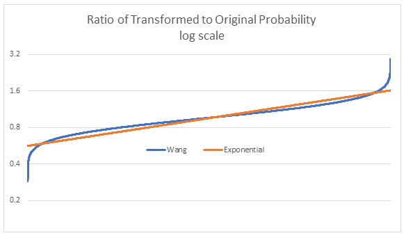
A transform that is less extreme in the tail is the exponential transform, given by q = [exp(pb) – 1] / [exp(b) – 1] for some b. These two transforms can be compared by looking at the ratio of q/p for transforms that give the same transformed mean. Below is an example from 50,000 simulations of gamma-distributed losses:
The transforms are similar over most of the probability range, but in the very far right tail, the Wang gives almost double the transformed probability.
Once capital is allocated, the business units are targeted the same return on capital, so the riskier ones have more capital and higher target profits on premium. Within units there could still be riskier and less risky classes of business, related for instance to limits and deductibles, or geography, etc. Usually for prices within units, it is better to use transforms designed for compound processes, which transform the frequency and severity with related transforms. I first heard of this idea in Thomas Møller’s paper “Stochastic orders in dynamic reinsurance markets” from the 2003 ASTIN Colloquium, available here. I found the paper hard to read but the transforms he was proposing involved first transforming the severity distribution. This puts more probability in the right tail, and reduces the probability for small losses. He then looks at the greatest reduction in probability for any loss, which is usually the limit at a loss of zero. He transforms the frequency to make its mean just enough higher to offset the greatest possible severity probability reduction.
Although not his focus, this approach solves a problem raised by a reviewer of my 1991 Astin paper on transformed distribution pricing – namely that deals can be constructed around the small losses – like deductible buy-backs – that would get a negative risk load. I found out recently that there is a wider literature on transforms for compound Poisson processes, but I haven’t look at that to date.
A simple transform like this that I give my students is for a Pareto severity with mean = b/(a – 1). Reducing the a parameter increases the severity, and does so more for higher limits and retentions. Since there is always a policy limit, it is fine if a < 1, for which the unlimited mean is infinite. This is the kind of transform that corresponds to actual market risk pricing to some degree anyway. The density limit at zero is a/b. Thus if a goes to a* < a, the probability near zero declines by a*/a, so you would increase the frequency mean by a/a*.
There is a growing body of literature on the application of probability transforms to the pricing of cat bonds. A lot of these are very public, with the cat model loss probabilities and the deal prices available. Thus it is a laboratory for transformed-mean pricing. Historically there are numerous papers that do this. One still developing paper is https://www.researchgate.net/publication/319583410_A_New_Class_of_Probability_Distortion_Operators_with_an_Application_to_CAT_Bonds
They look at transforms for compound Poisson processes and have a general framework as well.